A Review of Exemplar-based Image Completion

##Background Old pictures rots, sometimes scratch appears. Inpainting means to fix the deteriorated areas. This was used to be done by artists, but later with computers, automatic methods was invented, to fill the missing parts of the image.

Firstly, the PDE based algorithms. This class of methods based on pixels, not good at exploiting the higher level informations in an image. Since pixels contains extremely local features, it doesn’t work for large holes.

Exemplar-based methods use patches to find similar contents in the same image, and fill the missing regions with these contents. A higher level features can be expressed by patches, so it works fine for larger holes.

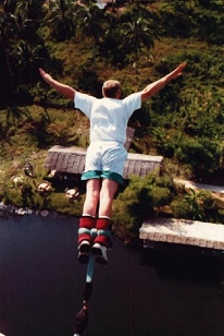
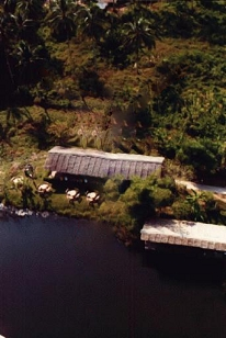
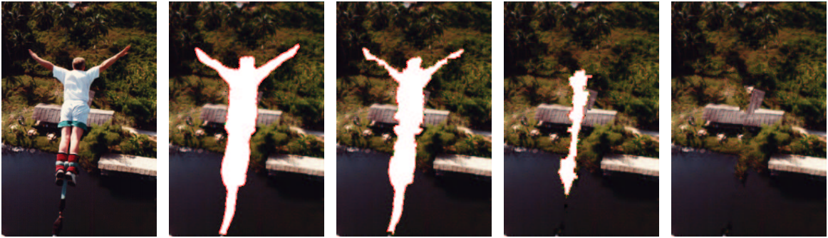
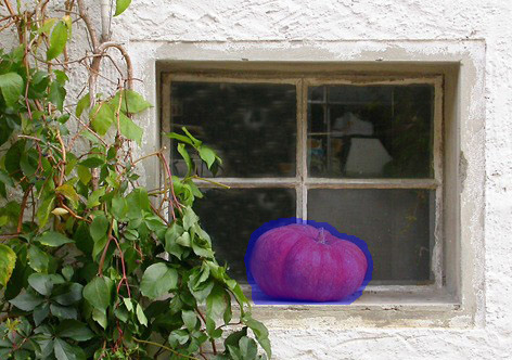
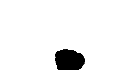
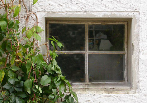
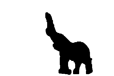
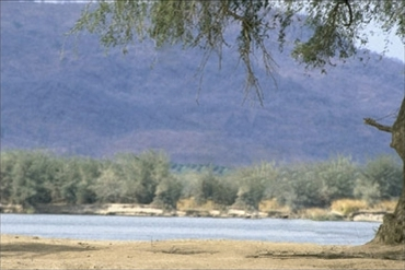
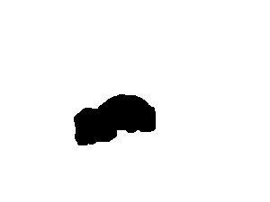
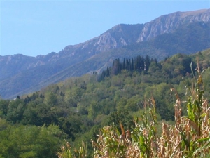
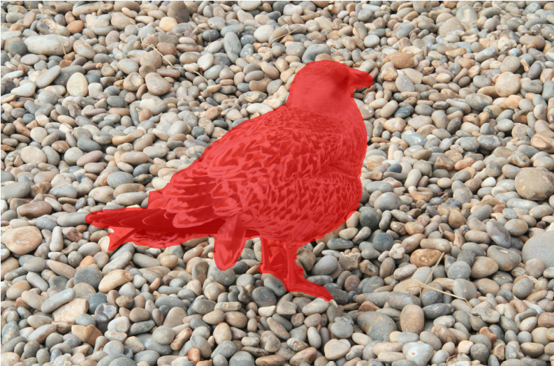
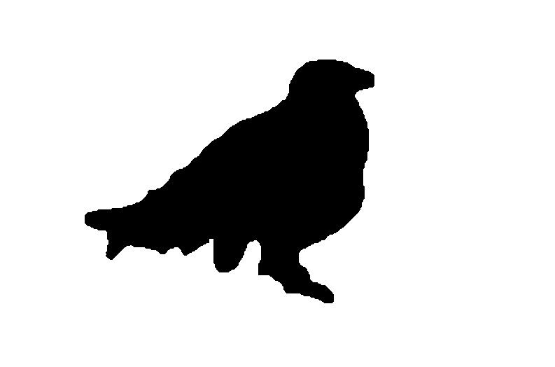
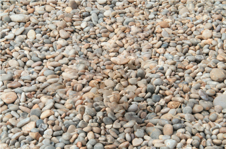
Following is a result of my implementation of an exemplar-based method based on TPAMI’14 paper¹, the image is from another paper².

Input	Mask	Result	Shift-Map

Although patch is a higher level feature than pixel (almost the same level as SIFT if you count the bits), it’s still not enough for complex contents because it doesn’t contain any semantic information. Some artifacts are just not artifacts until you put them in a view of semantics. In other words, the computer would think he works perfectly fine unless he can understand the object he’s dealing with.

For example the bungee result contains some repeated patterns on plants, which is weird for human. While the algorithm does not understand this, he took the repeating of the roof as an evidence that this area has a horizontal structure, which is true. But how could he know that the structure belongs to the man-made roof instead of the natural plants? He just cannot tell without any higher knowledges.

Thus some problems are just impossible to solve in the patch level. That’s why I’d say the further study of image completion must be on semantics. But that’s the future story, while this post focused on the patch based methods.

##Straightforward method A pioneer’s method is usually straightforward. CVPR’03 paper [Object Removal by Exemplar-Based Inpainting]² used a greedy approach. In each iteration, a patch was selected at the boundary of the missing regions, hence there are pixels in this patch that are already known. These pixels can be used to find the most similar patch which contains all known pixels. Then copy this intact patch to the selected one, and replace the missing pixels.

In each iteration some of the missing pixels were filled. By defining priorities based on contour and gradient, this method fill holes from boundary to central part, like peeling an onion.

Back to 2003, this was state of the art algorithm. It was simple, straightforward and works much better than PDE methods. But a greedy approach usually provides a suboptimal result. Moreover, I think this paper does not have a big picture. It seems right in every step, but did not give a mathematical explanation on what’s going on behind. In Variational Method’s view, what is the objective function to optimize?

Based on this, an interactive method³ was introduced to cope with structural contents. A curve was drawn to indicate the structure and dynamic programming was used to optimize the consistency of structural contents, also the searching space was largely reduced thanks to the manually work.

##Objective Function [Shift-Map Image Editing]⁴, an ICCV’09 paper provides a reasonable model. The image completion problem was defined as a Shift-Map optimization problem. Because exemplar-based method copies existed pixel to another place (in the hole), for each of the missing pixels, instead of asking what color it is, we can ask where should it come from. A Shift is a vector from the missing pixel to an existed one, the source pixel supposed to be copied to the missing place. Now a Shift-Map S can be defined on the missing areas, where S(p) is the shift vector at position p. Once we know S, we can find the source pixel at S(p), and copy it to replace p. Then the completion is done.

From all possible Shift-Maps we want a GOOD one, so we need to define GOOD. The objective function is a measurement of this goodness, which is defined as:

$$E(S) = \sum_{p \in H} E_d(p) + \lambda_1 \sum_{a,b \in N} E_s(a,b) + \lambda_2 \sum {p \in B} E_b(p)$$

where the data term $E_d$ measure the goodness of a single pixel, the smoothness term $E_s$ measure the goodness of the neighborhood relationship of two pixels, while boundary condition $E_b$ penalize the deviation of the boundary pixels. $\lambda$s are weights to balance their contributions.

$\lambda_2$ was set large to force the constraint. As for $\lambda_1$, we will later put it into $E_s$ and use different weights for different pixels’ smoothness term. See Smoothness term weights for details.

###Data term If we want to use S(p) to replace p, S(p) would better be a known pixel. If the shift at p shifts to another missing pixel, it does not help. Thus a desirable shift should lead us out of the hole.

Translate our requirements to mathematics:

$$E_d(p)= \begin{cases} 0, S(p) \notin H \\ +\infty, S(p) \in H \end{cases}$$

where $H$ is the hole, a set of all missing pixels. A big value was used instead of $+\infty$ in real life.

###Smoothness term The preferred Shift-Map is the one resulting to an image without seams, which means it’s hard to tell the reconstructed part from the original image. Seams can also be explained as the inconsistency of colors, so the objective function (the goodness measurement of S) must consider the consistency.

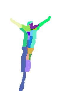
As optimal Shift-Map is shown in the result. Each color indicates a unique shift used to fill the missing pixels. It is perfectly seamless inside each of the colored regions, while the seams between them are unnoticeable because of the consistency.

To make it simple, we define consistency on adjacent pixels. Imagine that two adjacent pixels has the same shift, that will lead them to two source pixels which are adjacent too.

    +---+---+
    | a'| b'|
    +---+---+
    |   |   |
+---+---+---+
| a | b |
+---+---+

As the figure shows, adjacent pixels a and b, has the same shift (1, -2). Our image coordinates define top left as the origin.

In this condition, source pixels a’ and b’ will be used to replace a and b respectively. There will be no seam between a and b because a’ and b’ are adjacent by ground truth. The intact content must be seamless.

Generally things are not so perfect, adjacent pixels may take different shifts. However, even if they do, it does not always introduce a seam. For example:

            +---+---+
            | a1| b1|
+---+---+---+---+---+
| a2| b2|   |   |
+---+---+---+---+
        | a | b |
        +---+---+

Adjacent missing pixels a and b, has different shifts. Say a want to use a1 with shift (1, -2), while b want b2 with shift (-2, -1). The result puts a1 beside b2, which are not adjacent originally. A seam was introduced between them.

But what if we have a b2 with the same color of b1? Isn’t it equivalent to use a1 and b1 as before! So it’s still perfect. Actually as long as a1 b1 looks similar to a2 b2, the seam can be unnoticeable.

It seams like either a a1 closed to a2 or a b1 close to b2 is sufficient, do we really need to satisfy them both? In fact we are interesting with the similarity of contents, not the pixels, even 2 pixels are still too local to represent the contents. While in most of the papers they count both pixels, I recommend to use even more, as you will see.

So here comes the smoothness term:

$$E_s(a,b)=\sum_{x \in N(a,b) } \lambda_{(a,b)} Dist(I(x+S(a)) - I(x+S(b)))$$

where Dist is a similarity measurement for colors, usually $L_1$ or $L_2$ norm on RGB space, sometimes gradients are also involved to produce better performance. $I$ and $S$ are the image and Shift-Map, $N(a,b)$ a neighboring area around a,b. $\lambda_{(a,b)}$ is a weight depend on the position of pixel a and b, with the purpose to fix the position bias of the original function.

This definition differs from the original paper. The original smoothness term comes from SIGGRAPH’03 paper [Graphcut Textures: Image and Video Synthesis Using Graph Cuts]⁵ and is a special case of the above one where $N(a,b)$ takes no more pixels other than $a$ and $b$. With a larger neighborhood, it is more robust and easier to explain:

Since seam, or inconsistency, was introduced by adjacent pixels with different shifts. We can take some local pixels, and apply the different shifts to them and see how different they become. The total difference can measure the inconsistency. Or you can see it as to apply two shifts on both pixels and measure their differences not by the pixel itself but by the patch it centered.

In my implementation I sum the difference of pixels within radius 1 or 2.

###Boundary conditions The consistency is defined on two adjacent pixels, you can always copy an entire intact part to the missing regions and preserve the consistency. Then the central contents are all good except that they don’t fit in the environment, because of the seam between filled pixels and the intact ones.

Inconsistency must be penalized not only on missing areas, but also on boundaries. The same function can be applied on boundaries only that one of the two adjacent pixels is known now. To simplify the problem we can expand our unknown regions by 1 pixel and pretend that those boundary pixels are unknown, measure the inconsistency with the same Smoothness Term, and then constraint them to be close to their original value.

$$E_b(p) = Dist(I(p),I^*(p))$$

###Smoothness term weights There are still one problem. As the hole expand, boundary pixels grow linearly, while inner pixels grow quadratically. Thus to reduce the objective function, it is much easier to work on the inner pixels. The optimization will take that advantage, and overlook the importance of boundaries. An extreme result is to copy an entire region to the hole, put the all seams on the boundary. Since boundary pixels are minority, this may lead to a low function value, while the result is not plausible at all. The fact is that this function does not consider the importance and the weights of pixels.

In TPAMI’07 paper [Space-Time Video Completion]⁶, the same problem was addressed with a position based weight map. (Although they use a totally different objective function). The idea is to compensate the minority with larger weights. A distance transformation was a applied on the mask to figure out how far a pixel lies from the boundary. Closer pixels have larger weight for their smoothness terms.

The author use an exponential function as: $\lambda = \gamma ^d$. The reason is that exponential function has a recursive property to maintain the priority on each layer of the hole.

Similarly we can use

$$\lambda_{(a,b)}=\gamma ^{ {d_a+d_b} \over 2}$$

where $d_a$/$d_b$ are the distances from pixel a/b to the nearest boundary and $\gamma$ is experientially set to 1.3.

The [TPAMI’07]⁶ method was integrated with [Patch Match]⁷ in Adobe Photoshop CS5 known as Content-Aware Filling. It adopts an EM approach to optimize a different objective function and is very successful in applications. But it does not closely related to our implementation so I would save the details.

##Optimization Discretizing the unknown space, above function can be transformed to a discrete labeling problem, where each label represents a possible shift, and the solution is to assign labels to pixels. With the above objective function, the optimization belong to a well studied type: [Markov Random Field]⁸ (MRF) problems, where the objective function comprises data terms(depending on a single node/pixel) and smoothness terms(depending on two adjacent nodes/pixels). More complicated patterns are not considered. Our boundary condition can be combined to the data terms.

Optimization of MRF is typically NP-hard, but it can be efficiently approximated by [Belief Propagation]⁹ or Graphcuts. [Boykov-Kolmogorov algorithm]¹⁰ use an alpha-beta-swap approach to solve multi-labeled MRF problem by Graphcuts. They provide Matlab and C++ code.

After the Shift-Map guided copying & pasting, [Poisson Image Editing]¹¹ can be adopted to further improve the seams.

##Reduce the candidates There are too many possible shifts, not mention their combinations. [Shift-Map Image Editing]⁴ adopted a hierarchical approach but it’s still slow. PAMI’14 paper [Statistics of Patch Offsets for Image Completion]¹ use the prior to eliminate those improbable shifts and significantly improved the performance. As the author pointed out, unrelated shifts not only slow down the optimization, but also causes “overfitting”.

They use [Patch Match]⁷ to compute a NNF(Nearest Neighbor Field), where the Nearest Neighbor of a pixel was defined as the most similar patch to the patch centered at this pixel. Then the offsets from pixels to their nearest neighbors can be counted, and they found that the distribution of a natural image’s offsets are very sparse. 80% of the offsets dropped in 7% of all the possibilities. So they use the top 60 offsets as the candidate shifts for the previous Objective Function.

As shown in the optimal Shift-Map, there are only tens of shifts were used to reconstruct the missing contents, and results better than the onion peeling method.

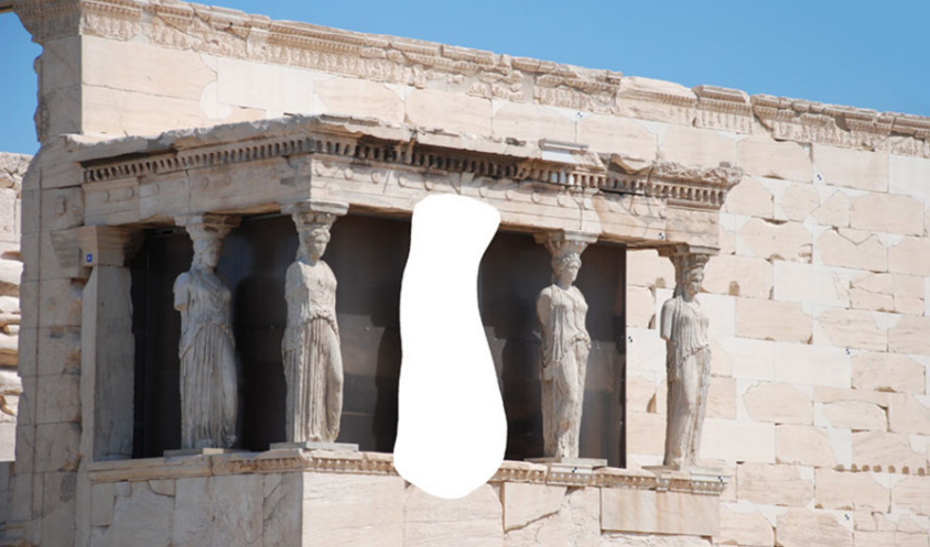
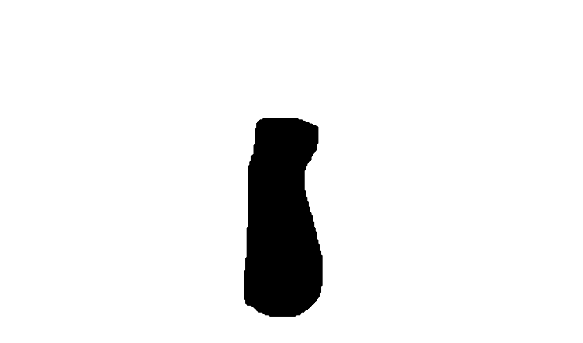
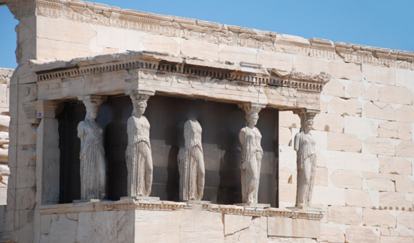
##More results:

Input	Mask	Result

##References: